(This Post is part of my 30 day Data Visualization Challenge – you can follow along using the ‘challenge’ tag!)

In noodling around with the different options of the qplot function (and there are plenty), I found myself going back and forth on the geom option – here’s one of the possible inputs, smooth, which takes us from yesterday’s graph to one of just very smooth lines, with a shading indicating the standard deviation of that particular collection of data:

Thoughts:
– This is a really interesting example of another case where we trade some visual precision for more visual utility – for example,that same graph using arguably more a more precise plotting of lines looks like a total, and useless, mess.
– The green line is particularly interesting, since it appears to plateau at a certain point – about the same place where it is the only remaining clarity.

Code:

library(ggplot2)
only.j <- subset(diamonds, color=="J")
j <- qplot(carat, price, data=only.j, color=clarity, geom=c("smooth"))
j

(This Post is part of my 30 day Data Visualization Challenge – you can follow along using the ‘challenge’ tag!)

After taking a look at the different colors of diamonds in a sample, I noticed that the diamonds colored “J” appeared to be unusual outliers. Following this tack, I created a subset of the larger diamond data set that contained _only_ the J colored diamonds – then, plotted that on the same carat/price graph we’ve seen, but with color now indicating the diamond’s clarity:

Thoughts:
– I also added a title, and started using variable names as I build around a data frame, which makes it much easier.
– We can see at least one of those vertical striations that we saw in the original data set.
– It looks like the outliers on the low-price-high-carat scale of the J-colored diamonds are larger but less valuable than their peers.
– This graph is a bit muddy, but we can for sure see what look like trends in clarity correlating with price as we go from orange to green to pink/purple.

Code:

library(ggplot2)
only.j <- subset(diamonds, color=="J")
j <- j <- qplot(carat, price, data=only.j, color=clarity, size=I(1.5))
j <- j + ggtitle("J-Color Diamond Clarity & Pricing")
j

(This Post is part of my 30 day Data Visualization Challenge – you can follow along using the ‘challenge’ tag!)

One of the neat things that ggplot2 can do is take a plot like yesterday’s, and automatically add a third dimension of data – for today I added the column “color,” which indicates the color of the actual diamond measured, as a “color” aesthetic:

Thoughts:
– Now we’re getting somewhere: we can see that yes, more carats tend to be associated with a higher price (with some outliers) but it also looks like certain colors (D,E, F) tend to be lower-priced and/or lower-carat. An interesting question might be to ask which of those factors is more strongly correlated with particular colors.
– We can also see that two of our outliers in this sample are both Js, so there may be interesting things to look into w/r/t that particular color.
– It might be nice to have some sort of drawn line or curve indicating a general trend, as well as maybe a trend per color?

Code:

library(ggplot2)
set.seed(1410)
dsmall <- diamonds[sample(nrow(diamonds),100),]
qplot(carat, price, data=dsmall, size=I(2), color=color)

(This Post is part of my 30 day Data Visualization Challenge – you can follow along using the ‘challenge’ tag!)

Yesterday’s visualization tried to handle this issue of data point density by reducing the actual size of the dots on the graph. The ggplot2 book (there’s a book!) recommends giving sampling a try. I’ve written a little about sampling and abstraction in the past – so let’s give it a try!

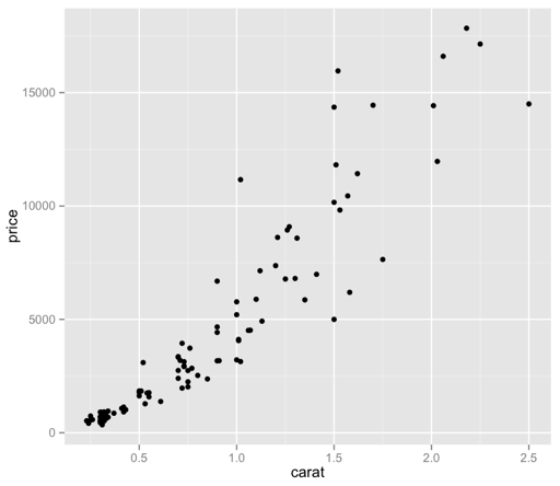
Now we’re cooking! I did have to bump the size of the points back up, as only 100 of those specks were not visually very helpful – but now we have a bit more of a visually intuitive sense of what we’re looking at, without guessing at the larger, imprecise ink blots.

It’s interesting, to me as a lapsed philosopher, that sampling (as an abstraction) necessarily means that we’re giving up precision (in the form of data points), but we’re doing so to gain another type of precision, that is, quick and accurate visual meaning. I’m dropping the Pros list – I’ll try to cover positive thoughts in the body of each Post.

Thoughts:
– What does it mean, though? We can see that there appears to be some sort of relationship between price and carat – how do the other factors come into play here? Are there other patterns at work?
– How can I make it prettier?
– It bothers me that “price” is vertical still. Dangit.

Code:

library(ggplot2)
set.seed(1410)
dsmall <- diamonds[sample(nrow(diamonds),100),]
qplot(carat, price, data=dsmall, size=I(2))