(This Post is part of my 30 day Data Visualization Challenge – you can follow along using the ‘challenge’ tag!)

After plotting the full dataset on a price vs. carat graph, one of the problems that occurred was this idea of dot density – proper data scientists probably have a more technical term for it. That is, with so many data points, it’s hard to tell how “deep” a dot is, since a visible dot may represent a larger number of data points.

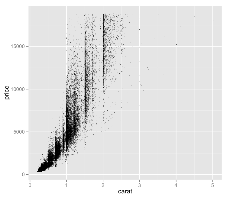
It seems like one possible solution would be to reduce the size of each dot – since each dot’s size may be causing it to visually encroach upon nearby data points, making the graph less visually useful. So, I tried that:

Pros:
– Offers a bit more nuance to the visual distribution of price vs. carat.
– Maintains the interesting vertical separations

Cons:
– This isn’t really a solution – with this number of data points, we still experience these big ink blots of imprecise “Well, there’s lots.” areas.
– It bothers me that “price” is vertical still. I forgot about that.
– The small size of the dots makes it tough to quickly distinguish outliers from a dirty laptop screen.

Code:

library(ggplot2)
qplot(carat, price, data=diamonds, size=I(1/3))

• Work